这是 @skotaro 在 2018 年发布的一篇关于 Matplotlib Artist 的通俗易懂的介绍,很适合作为官方教程的前置读物,故翻译于此,原文标题是 “Artist” in Matplotlib - something I wanted to know before spending tremendous hours on googling how-tos.。文中绝大部分链接都重定向到了最新版本的 Matplotlib 文档,还请读者注意。

毫无疑问 Python 里的 matplotlib 是个非常棒的可视化工具,但在 matplotlib 中慢慢调细节也是件很烦人的事。你很容易浪费好几个小时去找修改图里细节的方法,有时你连那个细节的名字也不知道的话,搜索起来会更加困难。就算你在 Stack Overflow 上找到了相关的提示,也可能再花几个小时根据需求来修改它。不过,只要了解了 matplotlib 图的具体组成,以及你可以对组件执行的操作,就能避开这些徒劳无益的工作。我想,我跟你们中的大多数人一样,做图时遇到的困难都是靠读 Stack Overflow 上那些 matplotlib 高手们的答案来解决的。最近我发现 官方的 Artist 对象教程 信息很丰富,有助于我们理解 matplotlib 的画图过程并节省调图时间1。本文里我会分享一些关于 matplotlib 里 Artist 对象的基本知识,以避免浪费数小时调图的情况出现。
本文的目的
我并不打算写那种“想要这个效果时你得如何如何”的操作说明,而是想介绍 matplotlib 中 Artist 的基本概念,这有助于你挑选搜索时的关键词,并为遇到的同类问题想出解决方案。读完本文,你应该就能理解网上那些海量的程序片段了。本文同样适用于用 seaborn 和 pandas 画图的人——毕竟这两个包只是对 matplotlib 的封装罢了。
内容
本文基本上是 我之前写的日文版文章 的英文版,内容主要基于 Artist tutorial 和 Usage Guide(原文发布时版本为 2.1.1)。
目标读者
这样的 matplotlib 使用者:
- 有能力根据需求画图,但要把图改到适合出版或展示的水平总是会很吃力(并且会为离预期效果就差那么一点而感到恼火)。
- 成功在 Stack Overflow 上找到了确切的解决方案,但对其工作原理仍然一知半解,也无法举一反三到其它问题上。
- 找到了好几个关于问题的提示,但不确定要选哪个。
环境
- Python 3.6
- matplotlib 2.2
%matplotlib inline
import matplotlib.pyplot as plt
import numpy as np
因为我开启了 Jupyter notebook 的行内绘图,所以本文略去了 plt.show()。
你需要注意的两种画图风格
在研究 Artist 对象之前,我想先提一下 plt.plot 和 ax.plot——或者说 Pyplot 和面向对象的 API——之间的差别。虽然官方推荐面向对象的 API 风格,但包括官方文档在内的很多地方还是存在许多 Pyplot 风格的例子和代码,甚至还有莫名其妙混用两种风格的,这显然会迷惑初学者。因为官方文档对此已经有过很好的注解,比如 A note on the Object-Oriented API vs. Pyplot 和 Coding Styles,所以我在这里只会简单解释一下。如果你需要关于这个话题的入门资料,我推荐官方教程:
面向对象的 API 接口
这是最为推荐的风格,一般以 fig, ax = plt.subplots() 或其它等价的语句开头,后跟 ax.plot、ax.imshow 等。实际上,这里的 fig 和 ax 就是 Artist。下面是几个最简单的例子:
fig, ax = plt.subplots()
ax.plot(x, y)
fig = plt.figure()
ax = fig.add_subplot(1,1,1)
ax.plot(x, y)
有些教程会用 fig = plt.gcf() 和 ax = plt.gca(),当你从 Pyplot 接口切换到面向对象接口时确实应该这么写,但有些纯 Pyplot 风格的代码里还写些无意义的 ax = plt.gca() ,这显然是无脑从面向对象代码里抄过来的。如果有意切换接口,那么使用 plt.gcf() 和 plt.gca() 并不是什么坏事。考虑到隐式切换可能会迷惑初学者,绝大部分情况下从一开始就显式地使用 plt.subplots 或 fig.add_subplot 就是最好的做法。
Pyplot 接口
这是一种 MATLAB 用户熟悉的画图风格,其中所有操作都是 plt.xxx 的形式:
# https://matplotlib.org/stable/tutorials/introductory/pyplot.html
def f(t):
    return np.exp(-t) * np.cos(2*np.pi*t)

t1 = np.arange(0.0, 5.0, 0.1)
t2 = np.arange(0.0, 5.0, 0.02)

plt.figure(1)
plt.subplot(211)
plt.plot(t1, f(t1), 'bo', t2, f(t2), 'k')

plt.subplot(212)
plt.plot(t2, np.cos(2*np.pi*t2), 'r--')
plt.show()
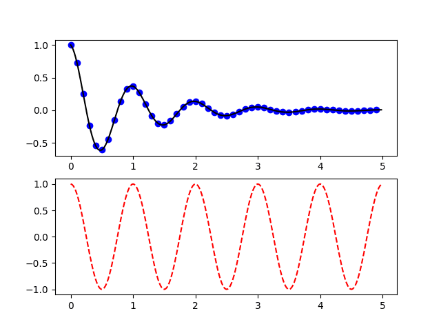
刚开始的时候你可能会觉得这种风格非常简单,因为不需要考虑你正在操作哪个对象,而只需要知道你正处于哪个“状态”,因此这种风格又被称作“状态机”。这里“状态”的意思是目前你在哪张图(figure)和哪张子图(subplot)里。正如你在 Pyplot tutorial 里看到的,如果你的图不是很特别复杂的话,这种风格能给出不错的效果。虽然 Pyplot 接口提供了许多函数来设置图片,但你可能不到一会儿就会发现这些功能还不够用,具体时间取决于你想要的效果,也许不到几小时、几天、几个月就会这样(当然运气好的话你不会碰到问题)。到了这一阶段你就需要转到面向对象接口了,这也是我推荐从一开始就使用面向对象接口的原因之一。不过当你需要快速验证或只想画点草图时,Pyplot 还是有挺有用的。
Matplotlib 的层级结构
在网上搜索几次后,你会注意到 matplotlib 有一个层级结构,由通常叫做 fig 和 ax 的东西组成。Matplotlib 1.5 的旧文档 里有张图能很好地解释这个:
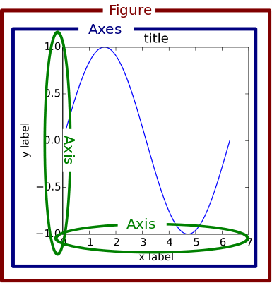
实际上,图中这三个组件是被称为“容器”的特殊 Artist(Tick 是第四种容器),我们后面还会再谈到容器。透过这种层级结构,前面举的简单例子会显得更加清晰:
fig, ax = plt.subplots() # 创建 Figure 和属于 fig 的 Axes
fig = plt.figure() # 创建 Figure
ax = fig.add_subplot(1,1,1) # 创建属于 fig 的 Axes
进一步查看 fig 和 ax 的属性能加深我们对层级结构的理解:
fig = plt.figure()
ax = fig.add_subplot(1,1,1) # 创建一个空的绘图区域
print('fig.axes:', fig.axes)
print('ax.figure:', ax.figure)
print('ax.xaxis:', ax.xaxis)
print('ax.yaxis:', ax.yaxis)
print('ax.xaxis.axes:', ax.xaxis.axes)
print('ax.yaxis.axes:', ax.yaxis.axes)
print('ax.xaxis.figure:', ax.xaxis.figure)
print('ax.yaxis.figure:', ax.yaxis.figure)
print('fig.xaxis:', fig.xaxis)
fig.axes: [<matplotlib.axes._subplots.AxesSubplot object at 0x1167b0630>]
ax.figure: Figure(432x288)
ax.xaxis: XAxis(54.000000,36.000000)
ax.yaxis: YAxis(54.000000,36.000000)
ax.xaxis.axes: AxesSubplot(0.125,0.125;0.775x0.755)
ax.yaxis.axes: AxesSubplot(0.125,0.125;0.775x0.755)
ax.xaxis.figure: Figure(432x288)
ax.yaxis.figure: Figure(432x288)
--------------------------------------------------------------------------------
AttributeError                            Traceback (most recent call last)
<ipython-input-21-b9f2d5d9fe09> in <module>()
      9 print('ax.xaxis.figure:', ax.xaxis.figure)
     10 print('ax.yaxis.figure:', ax.yaxis.figure)
--------> 11 print('fig.xaxis:', fig.xaxis)

AttributeError: 'Figure' object has no attribute 'xaxis'
根据这些结果我们可以归纳以下几条关于 Figure、Axes 和 Axis 层级结构的规则:
Figure知道Axes,但不知道Axis。Axes同时知道Figure和Axis。Axis同时知道Axes和Figure。Figure可以容纳多个Axes,因为fig.axes是一个由Axes组成的列表。Axes只能属于一个Figure,因为ax.figure不是列表。- 基于类似的理由,
Axes只能有一个XAxis和一个YAxis。 XAxis和YAxis只能属于一个Axes,因而也只能属于一个Figure。
图中一切皆为 Artist
目前 Usage Guide 里并没有放解释层级结构的图,而是放了一张名为”剖析一张图(Anatomy of a figure)“的示意图2,同样信息量十足,阐述了一张图所含的全部组件3。
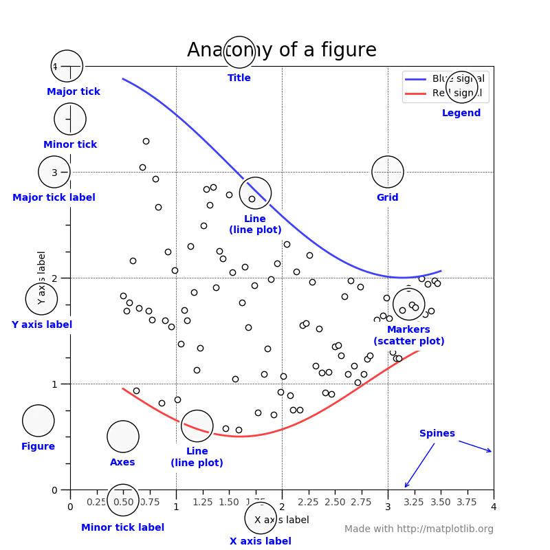
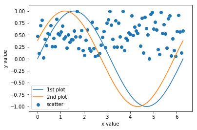
从代表数据的线条和点到 X 轴的小刻度和文本标签,图中每个组件都是一个 Artist 对象4。Artist 分为容器(container)和图元(primitive)两种类型。正如我在上一节写到的,matplotlib 层级结构的三个组件——Figure、Axes 和 Axis 都是容器,可以容纳更低一级的容器和复数个图元,例如由 ax.plot 创建的 Line2D、ax.scatter 创建的 PathCollection,或 ax.annotate 创建的 Text。事实上,连刻度线和刻度标签都是 Line2D 和 Text,并且隶属于第四种容器 Tick。
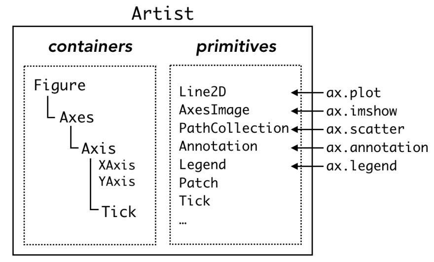
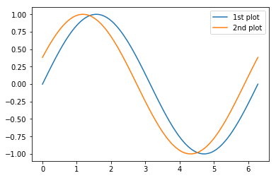
容器有许多存放各种图元的“盒子”(技术层面上就是 Python 列表),例如刚实例化的 Axes 对象 ax 会含有一个空列表 ax.lines,常用的 ax.plot 命令会往这个列表里添加一个 Line2D 对象,并在后台静默地进行相关设置。
x = np.linspace(0, 2*np.pi, 100)

fig = plt.figure()
ax = fig.add_subplot(1,1,1)
print('ax.lines before plot:\n', ax.lines) # 空的
line1, = ax.plot(x, np.sin(x), label='1st plot') # 往 ax.lines 里加 Line2D
print('ax.lines after 1st plot:\n', ax.lines)
line2, = ax.plot(x, np.sin(x+np.pi/8), label='2nd plot') # 再加一个 Line2D
print('ax.lines after 2nd plot:\n', ax.lines)
ax.legend()
print('line1:', line1)
print('line2:', line2)
ax.lines before plot:
 []
ax.lines after 1st plot:
 [<matplotlib.lines.Line2D object at 0x1171ca748>]
ax.lines after 2nd plot:
 [<matplotlib.lines.Line2D object at 0x1171ca748>, <matplotlib.lines.Line2D object at 0x117430550>]
line1: Line2D(1st plot)
line2: Line2D(2nd plot)
接下来概述一下这四种容器,表格摘自 Artist tutorial。
Figure
Figure 属性 |
描述 |
|---|---|
fig.axes |
含有 Axes 实例的列表(包括 Subplot) |
fig.patch |
用作 Figure 背景的 Rectangle 实例 |
fig.images |
含有 FigureImages 补丁(patch)的列表——用于显示 raw pixel |
fig.legends |
含有 Figure Legend 实例的列表(区别于 Axes.legends) |
fig.lines |
含有 Figure Line2D 实例的列表(很少用到,详见 Axes.lines) |
fig.patches |
含有 Figure 补丁的列表(很少用到,详见 Axes.patches) |
fig.texts |
含有 Figure Text 实例的列表 |
复数名的属性是列表,而单数名的则代表单个对象。值得注意的是属于 Figure 的 Artist 都默认使用 Figure 坐标,它 可以通过 Transforms 转换为 Axes 或数据的坐标,不过这个话题就超出本文的范围了。
fig.legend 和 ax.legend
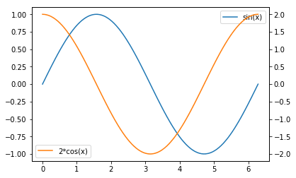
通过 fig.legend 方法 可以添加图例(legend),而 fig.legends 就是用来装这些图例的“盒子”。你可能会说“这有什么用?我们已经有了 ax.legend 啊。”区别在于二者的作用域不同,ax.legend 只会从属于 ax 的 Artist 里收集标签(label),而 fig.legend 会收集 fig 旗下所有 Axes 里的标签。举个例子,当你用 ax.twinx 画图时,单纯调用 ax.legend 只会创建出两个独立的图例,这通常不是我们想要的效果,这时 fig.legend 就派上用场了。
x = np.linspace(0, 2*np.pi, 100)

fig = plt.figure()
ax = fig.add_subplot(111)
ax.plot(x, np.sin(x), label='sin(x)')
ax1 = ax.twinx()
ax1.plot(x, 2*np.cos(x), c='C1', label='2*cos(x)')
# cf. 'CN' 形式的记号
# https://matplotlib.org/stable/tutorials/colors/colors.html#cn-color-selection

ax.legend()
ax1.legend()
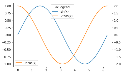
将两个图例合并在一起的经典技巧是,把两个 Axes 的图例句柄(handle)和标签组合起来:
# 在另一个 notebook 里执行这部分以显示更新后的图像
handler, label = ax.get_legend_handles_labels()
handler1, label1 = ax1.get_legend_handles_labels()
ax.legend(handler+handler1, label+label1, loc='upper center', title='ax.legend')
# ax1.legend 创建的图例仍然存在
fig
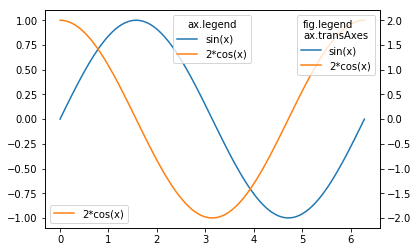
这个需求可以通过不给参数直接调用 fig.legend 来轻松解决(自 2.1 版本 引入5)。图例的位置默认使用 Figure 坐标,想把图例放在绘图框里面时会不太方便,你可以指定 bbox_transform 关键字改用 Axes 坐标:
fig.legend(loc='upper right', bbox_to_anchor=(1,1), bbox_transform=ax.transAxes, title='fig.legend\nax.transAxes')
fig
Axes
matplotlib.axes.Axes是 matplotlib 体系的核心。
这句话出自 Artist tutorial,说的非常正确,因为在 matplotlib 中数据可视化的重要部分都是由 Axes 的方法完成的。
Axes 属性 |
描述 |
|---|---|
ax.artists |
含有 Artist 实例的列表 |
ax.patch |
用作 Axes 背景的 Rectangle 实例 |
ax.collections |
含有 collection 实例的列表 |
ax.images |
含有 AxesImage 实例的列表 |
ax.legends |
含有 Legend 实例的列表 |
ax.lines |
含有 Line2D 实例的列表 |
ax.patches |
含有 Patch 实例的列表 |
ax.texts |
含有 Text 实例的列表 |
ax.xaxis |
matplotlib.axis.XAxis 实例 |
ax.yaxis |
matplotlib.axis.YAxis 实例 |
常用的 ax.plot 和 ax.scatter 等命令被称为”辅助方法(helper methods)“,它们会将相应的 Artist 放入合适的容器内,并执行其它一些杂务。
| 辅助方法 | Artist |
容器 |
|---|---|---|
ax.annotate |
Annotate |
ax.texts |
ax.bar |
Rectangle |
ax.patches |
ax.errorbar |
Line2D & Rectangle |
ax.lines & ax.patches |
ax.fill |
Polygon |
ax.patches |
ax.hist |
Rectangle |
ax.patches |
ax.imshow |
AxesImage |
ax.images |
ax.legend |
Legend |
ax.legends |
ax.plot |
Line2D |
ax.lines |
ax.scatter |
PathCollection |
ax.collections |
ax.text |
Text |
ax.texts |
下面这个例子展示了 ax.plot 和 ax.scatter 分别将 Line2D 和 PatchCollection 对象添加到对应列表里的过程:
x = np.linspace(0, 2*np.pi, 100)

fig = plt.figure()
ax = fig.add_subplot(1,1,1)
print('ax.lines before plot:\n', ax.lines) # 空的 Axes.lines
line1, = ax.plot(x, np.sin(x), label='1st plot') # 把 Line2D 加入 Axes.lines
print('ax.lines after 1st plot:\n', ax.lines)
line2, = ax.plot(x, np.sin(x+np.pi/8), label='2nd plot') # 加入另一条 Line2D
print('ax.lines after 2nd plot:\n', ax.lines)

print('ax.collections before scatter:\n', ax.collections)
scat = ax.scatter(x, np.random.rand(len(x)), label='scatter') # 把 PathCollection 加入 Axes.collections
print('ax.collections after scatter:\n', ax.collections)
ax.legend()
print('line1:', line1)
print('line2:', line2)
print('scat:', scat)
ax.set_xlabel('x value')
ax.set_ylabel('y value')
ax.lines before plot:
 []
ax.lines after 1st plot:
 [<matplotlib.lines.Line2D object at 0x1181d16d8>]
ax.lines after 2nd plot:
 [<matplotlib.lines.Line2D object at 0x1181d16d8>, <matplotlib.lines.Line2D object at 0x1181d1e10>]
ax.collections before scatter:
 []
ax.collections after scatter:
 [<matplotlib.collections.PathCollection object at 0x1181d74a8>]
line1: Line2D(1st plot)
line2: Line2D(2nd plot)
scat: <matplotlib.collections.PathCollection object at 0x1181d74a8>
不建议重复使用已经画好的对象
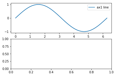
在知道了画好的对象会被存在列表里之后,你也许会灵机一动,尝试复用 Axes.lines 中的这些对象,即把它们添加到另一个 Axes.lines 列表中,以提高画图速度。Artist tutorial 里明确指出不推荐这样做,因为辅助方法除了创建 Artist 外还会进行很多其它必要的操作。随便测试一下就会发现这个思路确实行不通:
x = np.linspace(0, 2*np.pi, 100)

fig = plt.figure()
ax1 = fig.add_subplot(2,1,1) # 上面的子图
line, = ax1.plot(x, np.sin(x), label='ax1 line') # 创建一个 Line2D 对象
ax1.legend()

ax2 = fig.add_subplot(2,1,2) # 下面的子图
ax2.lines.append(line) # 尝试着把同一个 Line2D 对象用于另一个 Axes
就算是 add_line 方法也不行:
ax2.add_line(line)
ValueError: Can not reset the axes. You are probably trying to re-use an artist in more than one Axes which is not supported
报错信息表明,无论一个 Artist 是容器还是图元,都不能被多个容器同时容纳,这点也与前面提过的,每个 Artist 的父容器是单个对象而非列表的事实相一致:
print('fig:', id(fig))
print('ax1:', id(ax1))
print('line.fig:', id(line.figure))
print('line.axes:', id(line.axes))
fig: 4707121584
ax1: 4707121136
line.fig: 4707121584
line.axes: 4707121136
理论上如果你以合适的方式把所有必要的操作都做好了,应该就行得通,但这就完全偏离了只是想向列表追加一个对象的初心,这么麻烦的事还是别做了吧。
Axis
Axis 以 XAxis 和 YAxis 的形式出现,虽然它们只含有与刻度和标签相关的 Artist,但若想细调还总得上网搜搜该怎么做,有时这会耗掉你一个钟头的时间。我希望这一小节能帮你快速搞定这事。
Artist tutorial 里 Axis 不像其它容器那样有表格,所以我自己做了张类似的:
Axis 属性 |
描述 |
|---|---|
Axis.label |
用作坐标轴标签的 Text 实例 |
Axis.majorTicks |
用作大刻度(major ticks)的 Tick 实例的列表 |
Axis.minorTicks |
用作小刻度(minor ticks)的 Tick 实例的列表 |
在前面 Axes 容器的例子里我们用到了 ax.set_xlabel 和 ax.set_ylabel,你可能认为这两个方法设置的是 Axes 实例(ax)的 X 和 Y 标签,但其实它们设置的是 XAxis 和 YAxis 的 label 属性,即 ax.xaxis.label 和 ax.yaxis.label。
xax = ax.xaxis
print('xax.label:', xax.label)
print('xax.majorTicks:\n', xax.majorTicks) # 七个大刻度(从0到6)和两个因为出界而看不到的刻度
print('xax.minorTicks:\n', xax.minorTicks) # 两个刻度出界了(在图外面)
xax.label: Text(0.5,17.2,'x value')
xax.majorTicks:
 [<matplotlib.axis.XTick object at 0x117ae4400>, <matplotlib.axis.XTick object at 0x117941128>, <matplotlib.axis.XTick object at 0x11732c940>, <matplotlib.axis.XTick object at 0x1177d0470>, <matplotlib.axis.XTick object at 0x1177d0390>, <matplotlib.axis.XTick object at 0x1175058d0>, <matplotlib.axis.XTick object at 0x1175050b8>, <matplotlib.axis.XTick object at 0x117bf65c0>, <matplotlib.axis.XTick object at 0x117bf6b00>]
xax.minorTicks:
 [<matplotlib.axis.XTick object at 0x117ab5940>, <matplotlib.axis.XTick object at 0x117b540f0>]
ax.set_xxx 方法是暂时性的
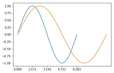
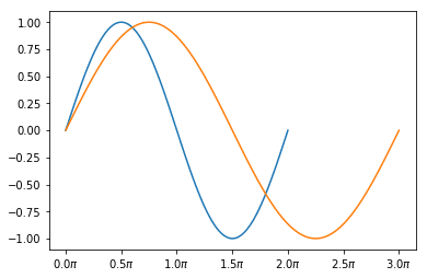
Axes 有很多形如 set_xxx 的辅助方法,可以修改 Axis 和 Tick 的属性和值。这些方法用起来非常方便,matplotlib 初学者遇到的大部分问题都可以借助其中一些方法来解决。需要注意 set_xxx 方法都是静态的,它们的修改结果并不会随之后的改动而更新。例如,你在第一次 plot 之后用 ax.set_xticks 把 X 刻度改得很合适,接下来第二次 plot 超出了第一次 plot 圈定的 X 范围,那么结果就会不合预期:
x = np.linspace(0, 2*np.pi, 100)

fig = plt.figure()
ax = fig.add_subplot(1,1,1)
line1, = ax.plot(x, np.sin(x), label='') # X 范围: 0 to 2pi
ax.set_xticks([0, 0.5*np.pi, np.pi, 1.5*np.pi, 2*np.pi])
line2, = ax.plot(1.5*x, np.sin(x), label='') # X 范围: 0 to 3pi
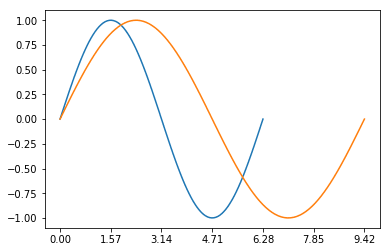
Ticker 帮你通通搞定
如果你不用 set_xxx 方法修改刻度参数,每次画上内容时刻度和刻度标签(tick label)会自动进行相应的更新。这归功于 Ticker,或者更准确点,formatter 和 locator。它们对于设置刻度来说极其重要,但如果你平时只靠复制粘贴 Stack Overflow 上的答案来解决问题,恐怕你对它们知之甚少6。让我们看看前一个例子里具体发生了什么吧:
译注:formatter 和 locator 似乎没有通用的译名,所以这里不译。
xax = ax.xaxis
yax = ax.yaxis
print('xax.get_major_formatter()', xax.get_major_formatter())
print('yax.get_major_formatter()', yax.get_major_formatter())
print('xax.get_major_locator():',  xax.get_major_locator())
print('yax.get_major_locator():',  yax.get_major_locator())
xax.get_major_formatter() <matplotlib.ticker.ScalarFormatter object at 0x118af4d68>
yax.get_major_formatter() <matplotlib.ticker.ScalarFormatter object at 0x118862be0>
xax.get_major_locator(): <matplotlib.ticker.FixedLocator object at 0x1188d5908>
yax.get_major_locator(): <matplotlib.ticker.AutoLocator object at 0x118aed1d0>
X 和 Y 轴都设置有 ScalarFormatter,因为这是默认的 formatter,并且我们也没有对其进行改动。另一方面,Y 轴设置的是默认的 AutoLocator,而 X 轴因为我们用 ax.set_xticks 改变了刻度的位置,现在被设置为 FixedLocator。顾名思义,FixedLocator 使用固定的刻度位置,即便之后画图区域变了也不会更新刻度位置。
接着让我们用 ax.set_xticks 以外的方法来改变上个例子中的 Ticker:
import matplotlib.ticker as ticker # 想使用 Ticker 必须要这一句
ax.xaxis.set_major_locator(ticker.MultipleLocator(0.5*np.pi)) # 每隔 0.5*pi 确定一个刻度
fig # 展示应用了新 locator 的 figure
再来看看 formatter:
@ticker.FuncFormatter # FuncFormatter 可以用作装饰器
def major_formatter_radian(x, pos):
    return '{}$\pi$'.format(x/np.pi) # 这可能不是显示弧度单位的刻度标签的最好方法

ax.xaxis.set_major_formatter(major_formatter_radian)
fig
好了,可能你还有想调整的地方,但我觉得讲到这儿已经够清晰了。
你可以在 matplotlib gallery 里学到更多:
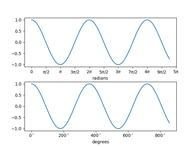
ax.plot 的 xunits 关键字
顺便一提,ax.plot 有个目前 还没有说明文档 的关键字 xunits,我自己是从来没用过,但你可以在 Gallery > Radian ticks 页面看到例子,更多关于 matplotlib.units.ConversionInterface 的内容请点 这里。
import numpy as np
from basic_units import radians, degrees, cos
from matplotlib.pyplot import figure, show

x = [val*radians for val in np.arange(0, 15, 0.01)]

fig = figure()
fig.subplots_adjust(hspace=0.3)

ax = fig.add_subplot(211)
line1, = ax.plot(x, cos(x), xunits=radians)

ax = fig.add_subplot(212)
line2, = ax.plot(x, cos(x), xunits=degrees)
Tick
终于,我们抵达了 matplotlib 层级结构的底部。Tick 是个很小的容器,主要容纳表示刻度的短线和表示刻度标签的文本。
Tick 属性 |
描述 |
|---|---|
Tick.tick1line |
Line2D 实例 |
Tick.tick2line |
Line2D 实例 |
Tick.gridline |
用作网格的 Line2D 实例 |
Tick.label1 |
Text 实例 |
Tick.label2 |
Text 实例 |
Tick.gridOn |
控制是否画出网格线的布尔量 |
Tick.tick1On |
控制是否画出第一组刻度线的布尔量 |
Tick.tick2On |
控制是否画出第二组刻度线的布尔量 |
Tick.label1On |
控制是否画出第一组刻度标签的布尔量 |
Tick.label2On |
控制是否画出第二组刻度标签的布尔量 |
类似于 Axis,Tick 同样以 XTick 和 YTick 的形式出现。第一组和第二组分别指上边和下边的 XTick,以及左边和右边的 YTick,不过第二组默认是隐藏的。
xmajortick = ax.xaxis.get_major_ticks()[2] # 上一张图里每隔 0.5 pi 出现的刻度
print('xmajortick', xmajortick)
print('xmajortick.tick1line', xmajortick.tick1line)
print('xmajortick.tick2line', xmajortick.tick2line)
print('xmajortick.gridline', xmajortick.gridline)
print('xmajortick.label1', xmajortick.label1)
print('xmajortick.label2', xmajortick.label2)
print('xmajortick.gridOn', xmajortick.gridOn)
print('xmajortick.tick1On', xmajortick.tick1On)
print('xmajortick.tick2On', xmajortick.tick2On)
print('xmajortick.label1On', xmajortick.label1On)
print('xmajortick.label2On', xmajortick.label2On)
xmajortick <matplotlib.axis.XTick object at 0x11eec0710>
xmajortick.tick1line Line2D((1.5708,0))
xmajortick.tick2line Line2D()
xmajortick.gridline Line2D((0,0),(0,1))
xmajortick.label1 Text(1.5708,0,'0.5$\\pi$')
xmajortick.label2 Text(0,1,'0.5$\\pi$')
xmajortick.gridOn False
xmajortick.tick1On True
xmajortick.tick2On False
xmajortick.label1On True
xmajortick.label2On False
得益于各种辅助方法、Ticker 和 Axes.tick_params,基本上我们不需要直接操作 Tick。
是时候自定义你的默认样式了
来瞧瞧默认样式的一系列参数吧。
Tutorials > Customizing matplotlib > A sample matplotlibrc file
我猜你现在应该能理解各个参数的作用,并且知道参数具体作用于哪个 Artist 了,这样一来以后搜索时可以节省大把时间7。除了通过创建 matplotlibrc 文件来自定义默认样式,你还可以直接在代码开头写上这种语句:
plt.rcParams['lines.linewidth'] = 2
去看文档吧(又来了)
有些读者可能对 matplotlib 文档印象不好,我也承认,从那么长的文章列表里为你的问题找出一个合适的例子还挺难的。但其实文档自 2.1.0 版本以来改进了很多8,当你对比改进前后的同一页面时尤为明显。
| 2.1.0(2017 年 10 月) | 2.0.2(2017 年 5 月) |
|---|---|
| Gallery, Tutorials | Matplotlib Examples, Thumbnail gallery |
| Overview | Overview |
我推荐你看一眼 最新的 gallery 和 Tutorials,现在的效果真的很赏心悦目。
译注:神秘的是,2.1.0 开始 Examples 页面改名为 Gallery,而到了 3.5.0,又改回 Examples 了,但网址里还是写的 gallery。
感谢你读到这里,尽情享受 matplotlib 绘图(和网络搜索)吧 📈🤗📊
封面图来自 Caleb Salomons on Unsplash
-
没错,如果你不是那种使用前连教程都不读的懒人,那么教程总会是信息丰富和大有裨益的。其实几年前我刚开始用 matplotlib 画图时好像就试过读
Artist的文档,但可以确定的是,我当时心里肯定想着“好吧,这不是给我这种用户读的”(也有可能当时读的不是现在的官方教程)。 ↩︎ -
制作这张图的示例代码在 https://matplotlib.org/stable/gallery/showcase/anatomy.html。 ↩︎
-
当然还存在其它的
Artist,想一览总体概貌的读者可以从 这个页面 入手。点击每个Artist的名字能看到更多说明。 ↩︎ -
技术上来说,在 matplotlib 里,艺术家(
Artist)会把你美丽的数据绘制在画布(canvas)上。这修辞还蛮可爱的。 ↩︎ -
以前版本里的
fig.legend要比现在难用,因为必须显式给出图例句柄和标签作为参数(据 文档 2.0.2)。 ↩︎ -
当你不满于
set_xxx之类的方法,更进一步搜索刻度相关的设置时,将会遇到许多使用 formatter 和 locator 的程序片段——然后摸不着头脑,只能放弃在自己的问题里应用它们(其实几个月前的我就是这样的)。 ↩︎ -
或者你可以像我一样用省下的时间继续钻研 matplotlib。 ↩︎
-
关于改进文档有多困难,这儿有篇不错的资料可以读读:Matplotlib Lead Dev on Why He Can’t Fix the Docs | NumFOCUS ↩︎